Chapter 3 gave a brief introduction of the most frequently used options within \(\tau\)-Argus. In this section a more detailed description of the program by menu-item is presented. In Chapter 5 some general descriptions are given.
Compared with the previous versions of \(\tau\)-Argus (before 4.0 and before the Open Source version) the main window of \(\tau\)-Argus looks rather different. A window with the unsafe combinations by variable and by code was presented. This information however was seldom used and the main focus of the users of \(\tau\)-Argus was on the table itself. So from version 4.0 onwards the main window of \(\tau\)-Argus will show the table(s) itself.
4.2 Viewing the table
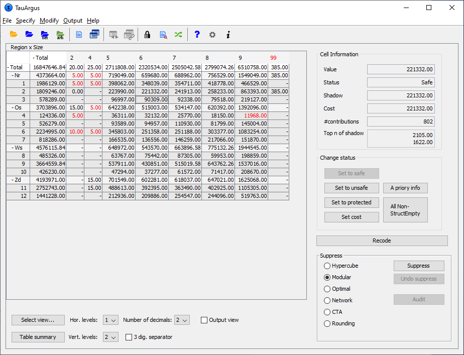
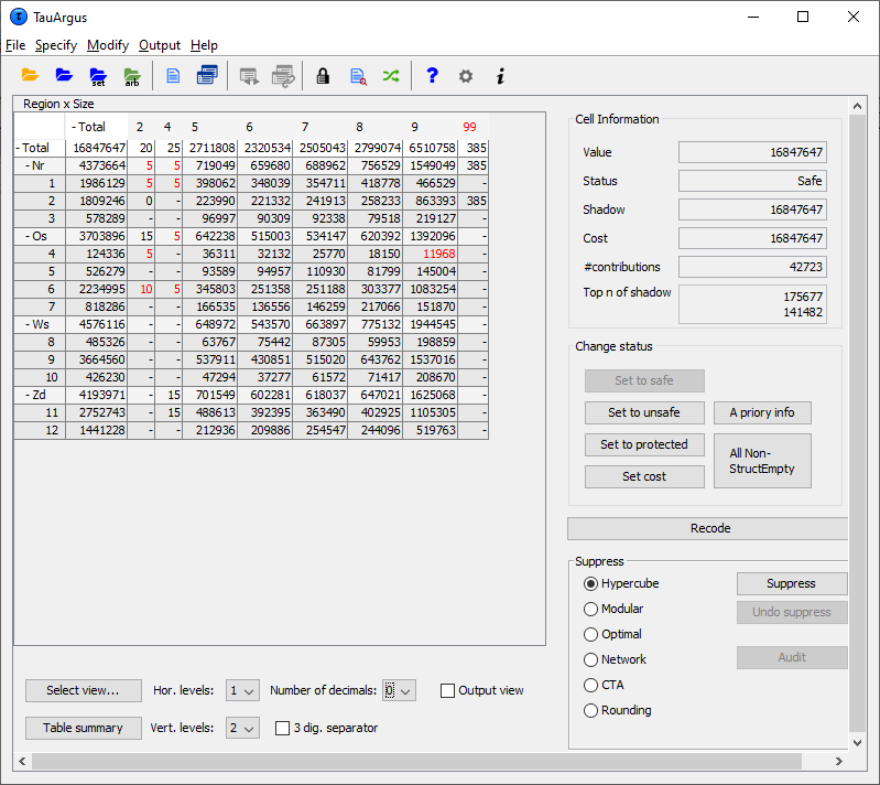
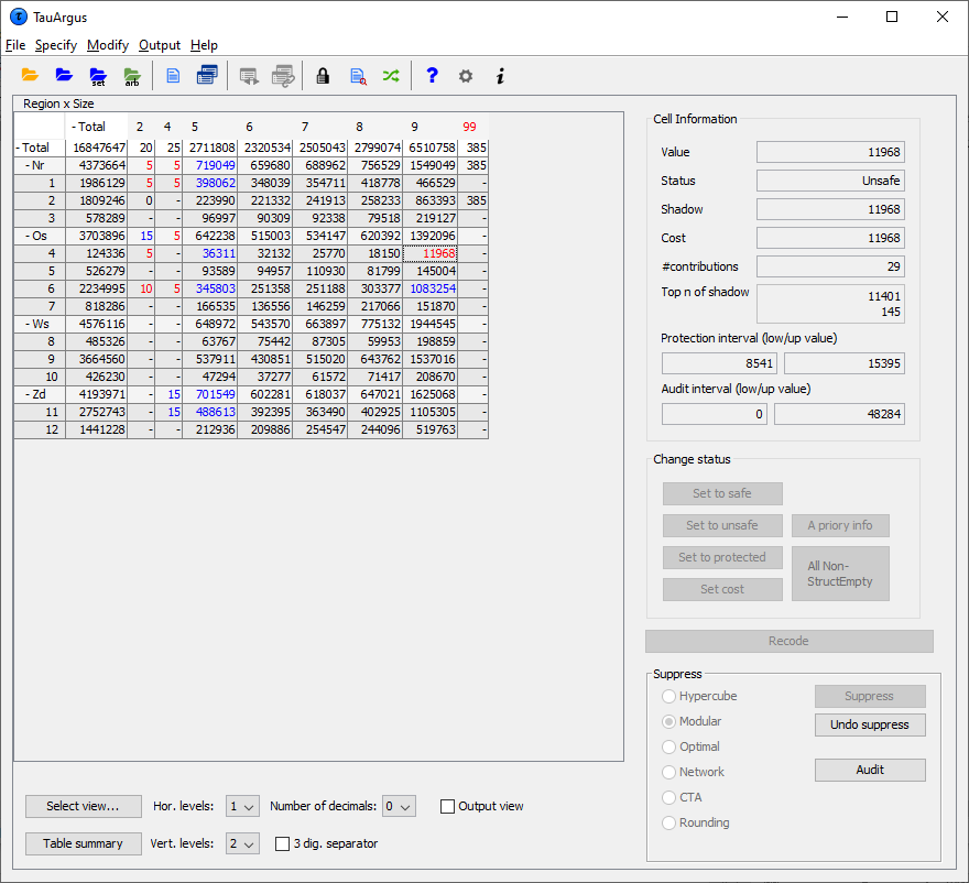
On the left side the table itself is shown in a spreadsheet view. Safecells are black, unsafe cells (those failing the primary suppressionrule) are red. In this example there are 12 unsafe cells and byviewing the table the user can now see the actual cells that areunsafe. Any secondary suppressed cells are shown in blue (there are none atthis stage, in this example) and empty cells have a hyphen (-). Thetwo check-boxes on the left-bottom give some control over the layout.
If the 3-digit separator box at the bottom is checked, the window > will show the cell-values, using the 3 digits separator to give a > more readable format.
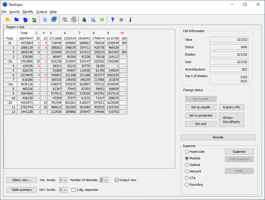
The Output view shows the table, with all the suppressed cells > replaced by an ‘X’; this is how the safe table will be published, > but without the colours distinguishing between primary and > secondary suppressions.
 For some windows, the complete table cannot be seen on the screen. Inthese cases there will be scrollbars at the bottom and the right ofthe table above, which can be used to display the unseen columns. For large tables one does not want to see the whole table on thescreen, which is virtually impossible. Therefore \(\tau\)-Argus will showonly the first two levels of the hierarchal structures. If you want tosee more you can open and close certain parts of the table by clickingon the codes with a ‘+’ or “-”sign. This works similar to the way youopen and close certain parts in the Windows explorer. Via ‘ChangeView’ at the bottom of the screen you can also select the level ofeach hierarchy you want to see both horizontally and vertically. Example of a 3-dimensional table 3-dimensional tables cannot be displayed as a whole. \(\tau\)-Argus can onlyshow a 2-dimensional layer of the table. So for higher dimensionaltable two variables are selected to be show. For the other variablescombo-boxes are shown. These combo-boxes allow for the selection of aspecific layer of the table. Just select the corresponding code andthat layer will be shown. If you want to see another combination of two explanatory variables,go to “Select view” at the bottom of the window. See section[4.2.7].
 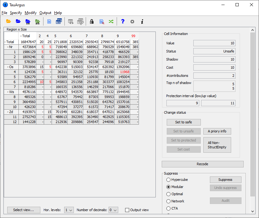 ****Additional information in the View Table window**** Clicking on a cell in the main body of the table makes informationabout this cell visible in the Cell Information**** pane****.**** Here, the following information can be seen:
the cell-value
the cell status
the value of cost variable
the value of the shadow variables
the number of contributors
the values of the largest contributors of the shadow variable ****In addition for a primary unsafe cell also the required lower andupper protection levels are shown. If you put your mouse over thisvalue, also the lower and upper protection as a distance to the cellvalue is shown together with the same value as a percentage. **** Information about the Holding level and the Request protectionvariable are also displayed here. The status of the cell can be:
Safe: Does not violate the safety rule
Safe (from manual): manually made safe during this session
Unsafe: According to the safety rule
Unsafe (request): Unsafe according to the Request rule.
Unsafe (frequency): Unsafe according to the minimum frequency rule.
Unsafe (from manual): manually made unsafe during this session (see > ‘Change Status’ below).
Protected: Cannot be selected as a candidate for secondary cell > suppression (see ‘Change Status’ below).
Secondary: Cell selected for secondary suppression.
Secondary (from manual): Unsafe due to secondary suppression after > primary suppressions carried out manually (see ‘Change Status’ and > ‘Secondary suppressions’ below).
Empty: No records contributed to this cell and the cell cannot be > suppressed. Change Status The second pane (‘Change Status’) on the right will allow the user tochange the cell–status.
Set to Safe: A cell, which was unsafe, e.g. due to the safety rules > is made safe by the user.
Set to Unsafe: A cell, which has passed the safety rules is made > unsafe by the user. Hence the manual safety margin is applied
Set to Protected: A safe cell is set so that it cannot be selected > for secondary suppression. Note: use this option with care as > the result might be that no solution can be found. Alternatively > consider to set the cost-variable to a very high value.
Set Cost: Change the cost function for a cell.
4.2.1 A priori info
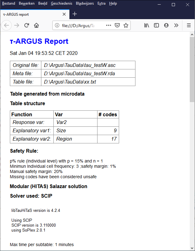
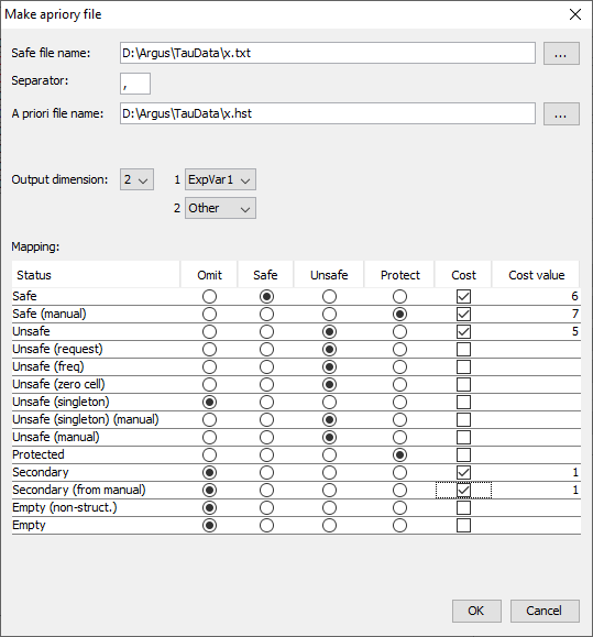
This option allows you to feed \(\tau\)-Argus a list of cells where thestatus of the standard rules can be overruled. E.g. a cell must bekept confidential or not for other reasons that just because of thesensitivity rules. By modifying the cost-function you can influencethe selection of the secondaries. E.g. the cells suppressed last yearcan get a preference for the suppression this year by giving this cella small value for the cost-function. The option ‘Expand trivial levels’ is important. Often in a table withhierarchies, some levels in a hierarchy break down in only one lowerlevel. This implies that there are different cells in a table whichare implicitly the same. Changing the status of one of them might leadto inconsistencies and serious problems. E.g. one if the two is unsafeand the other is protected, the solution is impossible. If you selectthe option ‘Expand trivial levels’, τ‑argus will always modify allcells that are the same if you modify one of them. The format of the file is free format. The separator can be chosen. The format is: Code of first spanning variable, Code of second spanning variable,…,Status of cell (u = unsafe, p = protected (not to be suppressed), s =safe). Also the cost-function can be changed here for a cell. This will makethe cell more likely to become secondary cell suppression, when thevalue is low, or less likely when the value is high. Normally the sensitivity rules will also give the required protectionlevels for unsafe cells. But sometimes, e.g. in the case of ‘manualunsafe cells’ the user might want to specify the required protectionlevel different for a standard percentage. After the keyword ‘pl’, thelower and upper protection levels can be given for a specific cell.Note that the protection levels will always have to be positive, asthey are considered as distances from the cell-value. A full description of the apriori file is given in section[5.6]. Nr, 4, u Zd, 6, p 5, 5, c, 1 Zd, 5, pl, 100, 200 When the apriori file has been applied \(\tau\)-Argus will show an overviewof the changes that have been made to the table. 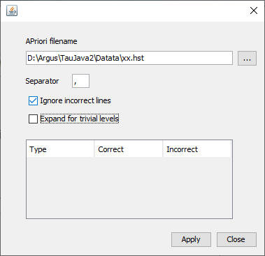
4.2.2 Global recoding
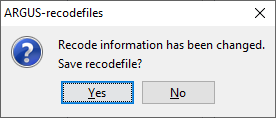
The recode button will open the recoding options. Recoding is a verypowerful method of protecting a table. Collapsed cells tend to havemore contributors and therefore tend to be much safer. Recoding a variable always starts with the original codes. It is notpossible to refine a recoding. If required you must start with acomplete new recoding. ****Recoding a non-hierarchical variable**** There is a clear difference in recoding a hierarchical variablecompared to a non-hierarchical variable. In the non-hierarchical case the user can specify a global recodingmanually. Either enter the recoding described below manually or readit from a file. The default extension for this file is .GRC. Detailscan also be found in section [5.4]. 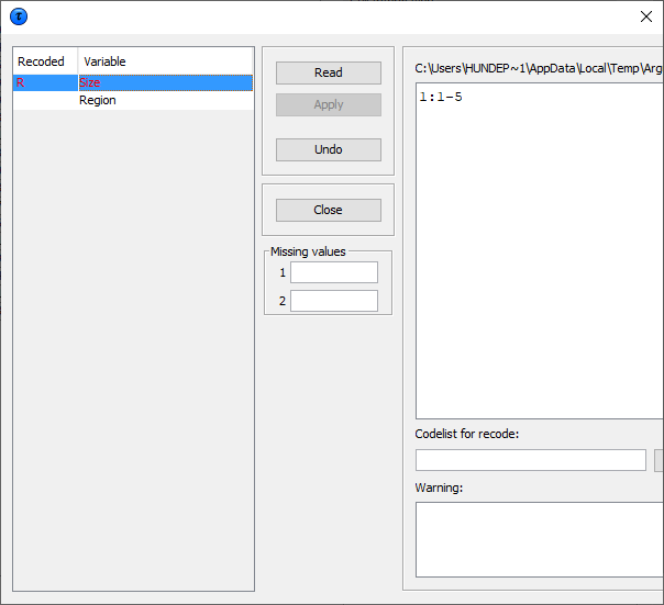 There are some standards about how to specify a recode scheme. Always the new code is specified first followed by a colon (`:`).After that the set of old codes to be collapsed into the new code isspecified. All codelists are treated as alphanumeric codes. This means thatcodelists are not restricted to numerical codes only. However, thisalso implies that the codes '01' and ' 1' are considered differentcodes and also 'aaa' and 'AAA' are different. In a recoding schemethe user can specify individual codes separated by a comma (,) orranges of codes separated by a hyphen (-). The range is determined bytreating the codes as strings and using the standard stringcomparison. E.g. `0111`< `11` as the `0` precedes the `1` and`ZZ’< `a` as the uppercase `Z` precedes the lowercase `a`.Special attention should be paid when a range is given without a leftor right value. This means every code less or greater than the givencode. In the first example, the new category 1 will contain all thecodes less than or equal to 49 and code 4 will contain everythinglarger than or equal to 150. Example:a variable with the categories 1,…,182 a possible recode isthen: 1: - 49 2: 50 - 99 3: 100 – 149 4: 150 – for a variable with the categories 01 till 10 a possible recode is: 1: 01 , 02 2: 03 , 04 3: 05 – 07 4: 08 , 09 , 10 An important point is not to forget the colon (:) if it is forgotten,the recode will not work.: 05,06,07 can be shortened to 3: 05-07. Additionally, changing the coding for the missing values can beperformed by entering these codes in the relevant textboxes. Also a new codelist with the labels for the new coding scheme can bespecified. This is entered by means of a codelist file. An example isshown here. (note, there are no colons is this file) 1,Groningen 2,Friesland 3,Drenthe 4,Overijssel 5,Flevoland 6,Gelderland 7,Utrecht 8,Noord-Holland 9,Zuid-Holland 10,Zeeland 11,Noord-Brabant 12,Limburg Nr,North Os,East Ws,West Zd,South Pressing the ‘Apply’ button will actually restructure the table. Thevariable concerned will be displayed in red and additionally an x isshown in front of the variable. If required, recoding can easily beundone by pressing 'undo recoding'. The window will return to theoriginally coding structure. If there is any error in the recodingsuch as certain codes not being found when pressing the ‘Apply’button, an error message will be shown at the bottom of the screen.Alternatively, a warning could be issued; e.g. if the user did notrecode all original codes, \(\tau\)-Argus will inform the user. This may havebeen the intention of the user, therefore the program allows it. Inthe above example a \(\tau\)-Argus message informs the user that 4 codes havenot been changed. At the end of the operation τ‑argus will ask you whether or not amodified recoding scheme must be saved or not.
  Once the ’Close’ button has been pressed, \(\tau\)-Argus will present thetable with the recoding applied. Recoding a hierarchical variable
 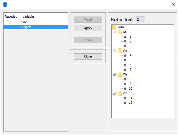 In the hierarchical case the code scheme is typically a tree. Toglobal recode a hierarchical variable requires a user to manipulate atree structure. The standard Windows tree view is used to present ahierarchical code. Certain parts of a tree can be folded and unfoldedwith the standard Windows actions (clicking on ‘+’ and ‘-’). The maximum level box at the top of the screen offers the opportunityto fold and unfold the tree to a certain level. Pressing the ‘Apply’ button will actually restructure the table. Ifrequired, a recoding may always be undone.
4.2.3 Secondary suppression
When the table is ready, the most commonly used method to protect atable is secondary cell suppression With suppress the table will be protected by causing additional cellsto be suppressed. This is necessary to make a safe table. Suppression Options There are a number of suppression options, which can be seen on thebottom right hand side of the window.
Hypercube
Modular
Optimal
Network
4.2.3.1 Hypercube
This is also known as the ghmiter method. The approach builds on thefact that a suppressed cell in a simple n‑dimensional table withoutsubstructure cannot be disclosed exactly if that cell is contained ina pattern of suppressed, nonzero cells, forming the corner points of ahypercube. Selecting the hypercube method will lead to the followingwindow being showed by \(\tau\)-Argus. ghmiter will select secondary suppressions that protect the sensitivecells properly against the risk of inferential disclosure, to someextent, if the user activates the option “Protection againstinferential disclosure required”. If the option is inactivated, onthe other hand, ghmiter will not check secondary suppressions to besufficiently large. For more explanation, and detailed information on the hypercube seesection [2.8]. The lower part of the window above enables the user to affect thesetting of two parameters, “Max sub-codelist size” and “Max sub-tablesize” that GHMITER uses for memory allocation. If the option ‘normal size’ is active, the default values mentionedbelow will be used. Ticking the option ‘large size’ will lead to asetting of 250 and 25000, respectively. “Max sub-codelist size” must exceed the largest maximum sub-codelistsize of all explanatory variables of the table. The maximumsub-codelist size of a (hierarchical) variable is the largest numberof categories on the same (hierarchical) level that contribute to thesame category on the (hierarchical) level just above. The defaultvalue for “Max sub codelist size” is 200. “Max sub-table size” must exceed the number of cells in the largestsubtable, e.g. the product of the maximum sub-codelist sizes takenover all explanatory variables. The default value is 6000. Note that we strongly recommend designing tables so that they fit the’normal’ setting, e.g. better think about restructuring the tablerather than using the ‘large’ option. The better approach (instead ofusing the ‘large’ option) would be to introduce a (more detailed)hierarchical structure into the table, because in this way the tablewill provide more information to the user. The Cancel button will bring you back to the main window, withoutprotecting the table.
4.2.3.2 Modular
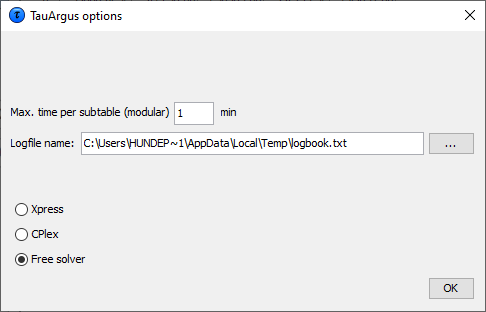
This partial method will break down the hierarchical table intoseveral non-hierarchical tables, protect them and compose a protectedtable from the smaller tables. As this method uses the optimisationroutines, an LP-solver is required: this can be either Xpress or cplexor a free solver. The routine used can be specified in the Optionsbox, this will be discussed later. After starting the modular procedure a little window will be shown.This allows to select three additional rules to be applied. At the endof section [2.10] more information on these three rulescan be found. 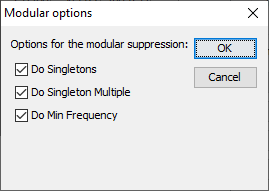
4.2.3.3 Optimal
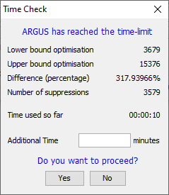
This method protects the (hierarchical) table as a single tablewithout breaking it down into smaller tables. As this method uses theoptimisation routines, an LP-solver is required: this can be eitherXpress or cplex or a free solver. The routine used can be specified inthe Options box, this will be discussed later. It is the responsibility of the users of \(\tau\)-Argus to apply for alicence for one of these commercial packages themselves. Informationon obtaining one of these licences will be found in a ‘read.me’ filesupplied with the software or on the CASC website. Almost the same window as in Modular is shown to select the 3additional rules; see above. 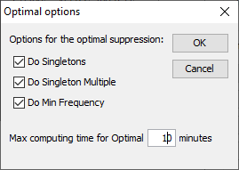 But a further question is asked. The question is ‘How much time do youallow the system to compute the optimal solution’. When the specified time limit has been reached τ‑argus will ask youwhat to do. This can be twofold, you allow τ‑argus to continue for anew amount of time, or not. The window below allows you to specifythis. Note that τ‑argus will check only at a specific location in a cyclewhether or not the time has elapsed.
4.2.3.4 Network
This is a Network Flow approach for large unstructured 2 dimensionaltables with only one hierarchy (the first variable specified). Theuser has the option of selecting an optimisation method (pprn andDykstra). Both optimisation methods are available free of anadditional licence. By default the Dykstra solution is advised. 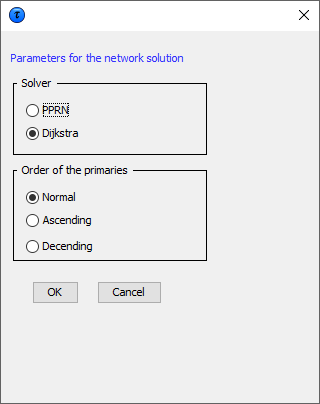 As the network solution is a heuristic to find an approximation of thereal optimal solution, it cannot be expected that always an optimalsolution is found. Nevertheless it is guaranteed that at least a goodfeasible solution is found in a relatively short time. The order inwhich the primaries are provided to the network algorithm couldinfluence the solution found. Therefore three options are available toorder the primaries.
4.2.3.5 After the suppression
After selecting one of the options and after clicking the Suppressbutton, \(\tau\)-Argus will run and display a protected table after informingthe user of the number of cells selected for secondary suppression andthe time taken to perform the operation. 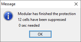 The secondary suppressed cells will be shown in blue.
 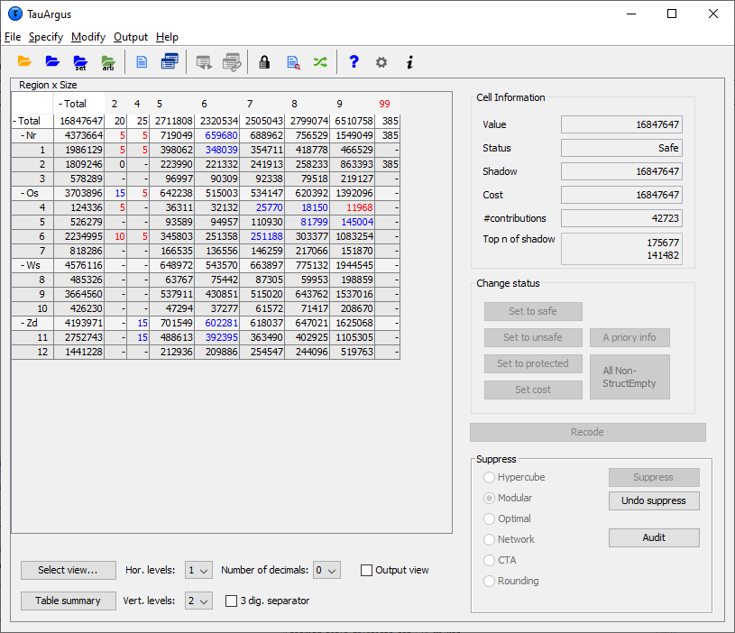 When the user is satisfied with the table it can be saved (see section[4.6.1] for the possible formats). Via the menuOutput|Save table you can specify the format and start the process ofsaving a table.
4.2.4 Controlled Tabular Adjustment
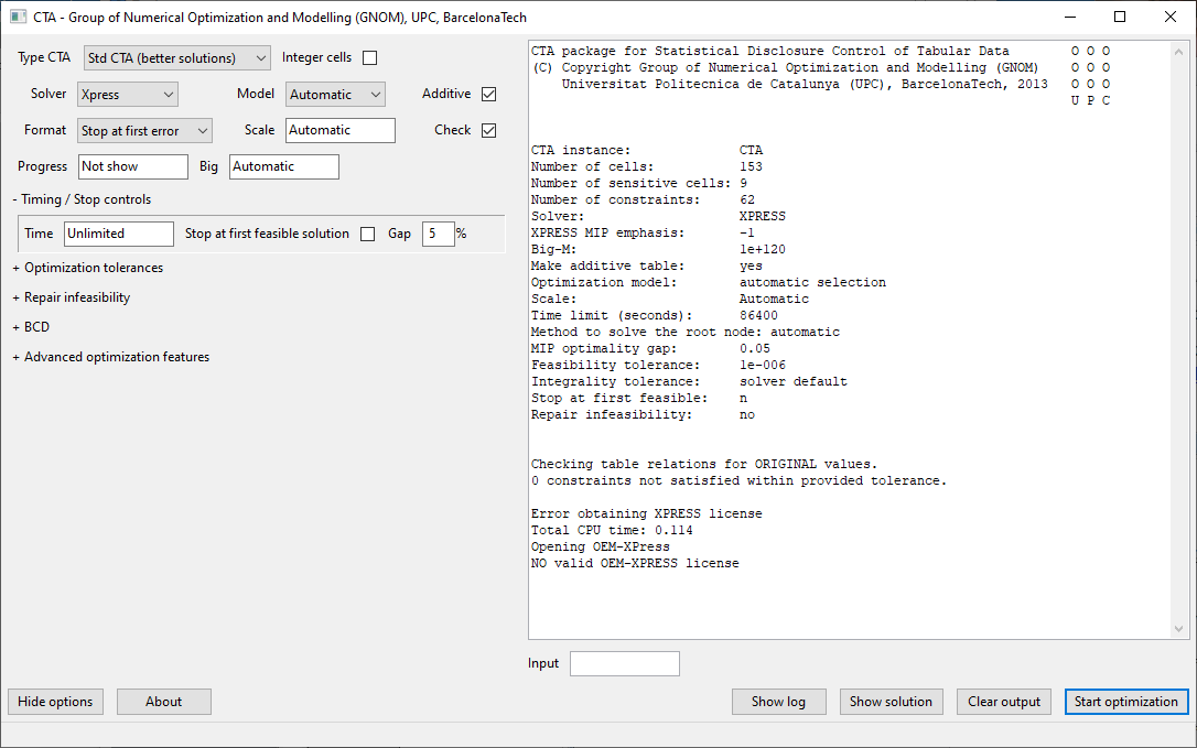
A method new in version 4.0 of \(\tau\)-Argus is a method called ControlledTabular Adjustment. Instead of suppressing a set of cells, a selectedset of cells is modified. The aim is to change the sensitive cellssuch that the cells are replaced by a value larger that the upperprotection level or smaller than the lower protection level. i.e. farenough away from the unsafe value.. And a set of safe cells ismodified such that the resulting table is additive again. Of course wetry to minimise the information loss. More information can be found in section [2.13]. We have implemented two variants. A standard version, suitable forgeneral cases, and an expert version for the specialists.  The standard version will run CTA without any further questions. The expert version will show the following window: You can e.g. selectthe solver and the type of CTA. We further refer to the detailed CTAdocumentation.
4.2.5 Controlled rounding
Controlled rounding (see Section [2.14] for details onthis method) requires a solver that allows you using the Mixed IntegerModel (MIP). Already in version 3 of τ‑argus we had access to MIP inXpress, thanks to the friendly cooperation of Dash Inc and later FICO.However the restricted version of the cplex licence we used in version3 of \(\tau\)-Argus did not have access to MIP. But from now on you can buy alicence for cplex including MIP. This allows you to use ControlledRounding with a new cplex licence. Also the free solver, soplex, can be used for Controlled Rounding. In general, rounding is more appropriate for frequency tables than formagnitude tables. The next figure shows the simple frequency table obtained from thetest data using the variable Size and Region. 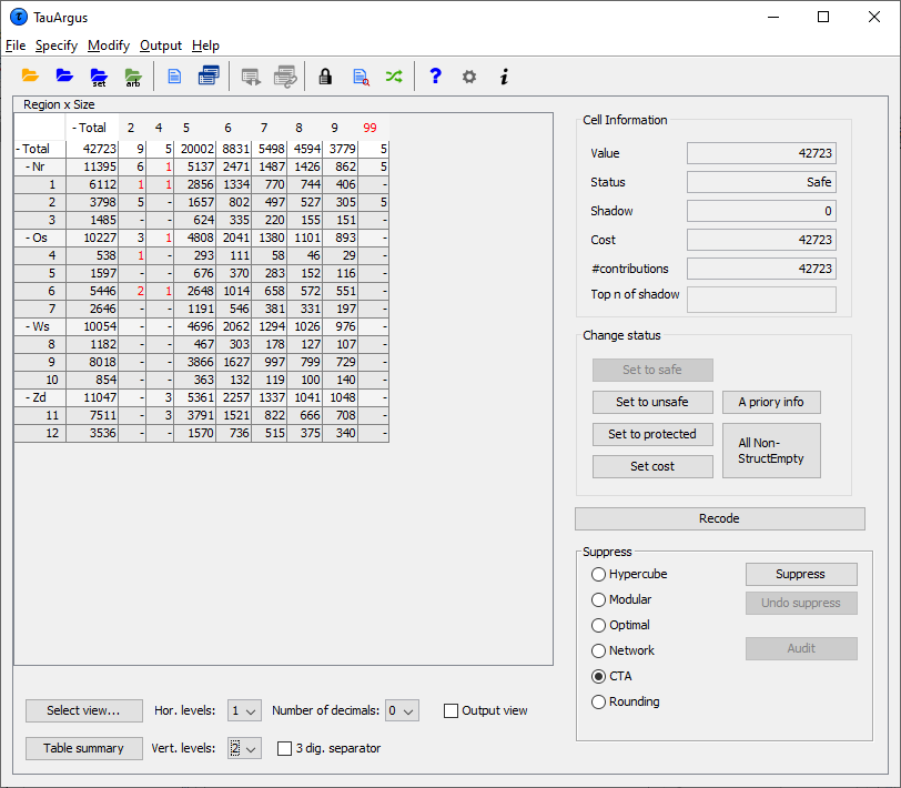 Rounding can be applied also to tables with no unsafe cells. Thechoice of the minimum threshold and whether zeros are safe or not hasan effect on the minimal possible rounding base, as it will beexplained in the Option paragraph. When rounding has been chosen and the round-button has been pressed,the following window will be shown. You can enter a few parameters. Rounding Options
 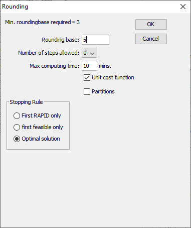 The controlled rounding window allows to set the following parameters:
Rounding Base
> Cell values will be changed to multiples of the base. The minimum > rounding base is equal to the maximum between the minimum > frequency threshold and twice the highest Protection Level set for > an unsafe cell (with the Dominance or p-q rule). See the Section > [2.2] for details on safety rules and section > [2.6] protection levels. If no rule is specified the > minimum base is 1. Rounding can be used to round a table for > “cosmetic” motives.Number of steps allowed
> This value specifies the maximum number of steps allowed in > order to find a feasible solution when a zero-restricted one does > not exist. The default value is 0, i.e. zero-restricted. Higher > values can be chosen by selecting the value from the drop-down > menu. Note that the higher the number of steps allowed the > lengthier is the search, hence the greater the risk of hitting the > time constraint. At any rate, if a zero-restricted solution > exists, this is the solution provided, whatever the number of > steps allowed.Max computing time
> This value determines the time after which the user is prompted > for a decision about continuing or stopping the search. The > default value is 20 minutes. When the maximum time is hit the user > is prompted to enter a new maximum time or to choose to terminate > the search.Partitions
> This option enables the partitioning of the table into sub-tables > corresponding to each category of the first spanning variable. > This option is recommended for tables with more than approximately > 150,000 cells. Partitioning can only be used in this version when > the first variable is non-hierarchical. The first variable should > be such that the sub-tables have maximum size of about 150,000 > cells and also trying to keep their number low; performance may be > improved by wisely choosing the partitioning variable. See Section > (rounding theory) for further details.Stopping Rule These options allow to control the quality of the rounded solution.The user can choose:
First Rapid
> The solution is obtained by rounding conventionally (to the > closest multiple of the base) the internal cells and then the > marginal values are obtained by addition. This solution is likely > to present several values that have a large distance from the > original values. This option should be used with extreme care and, > likely, when everything else fails;First feasible
> The solution provided is the first rounded one that has the > specified number of jumps, regardless of its optimality. This > means that there could exist other solutions that have a lower > overall distance from the original table. In many cases, when > optimality is not crucial, this solution is quite close to the > optimal one and it can be found in a shorter time;Optimal
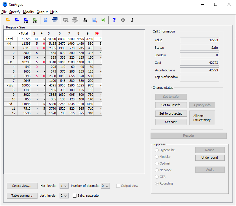
> This option provides the fully optimal controlled rounded > solution.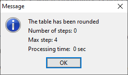 The rounded table The next figure shows the rounded table with the values rounded tomultiples of 5. Note that the values that were originally zero (henceempty cells denoted with a dash) are still shown as a dash while thevalues that have been rounded down to zero are shown as zeros.
4.2.6 The audit procedure
After the secondary cell suppression procedure has been carried outall cells should have been properly protected. Cell suppressionguarantees that unsafe cells cannot be estimated to a narrowerinterval that the required protection interval. The realised upper andlower bounds can be computed by solving two linear programmingproblems for each unsafe cell. This can be rather an effort doing itall manually, but the audit procedure will do this. Note that theModel solved by the audit procedure will check only for the requiredprotection levels, but not for the additional singleton protection.See also section [2.15]. The Audit option will only be active after secondary cell suppression.By activating the procedure all the linear programming problems forall unsafe (both primary and secondary) cell will be computed. Whencompleted a message will be showing whether all cells were protectedcorrectly. 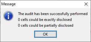 If in the unfortunate case the protection was not optimal according tothe audit procedure a list of problems will be shown. Also theproblematic cells will be highlighted. For each unsafe cell the realised lower and upper bounds will beshown. If you put your mouse on the value also the distance to thereal value and the corresponding percentage will be shown
4.2.7 The Options at the Bottom of the table
At the bottom of this window there are a few additional options. Theseoptions will be described here. Select View By clicking on Select View a dialog box below pops up. The user canspecify which variable is preferred in the row and the column. In thetwo-dimensional case, the table can only be transposed. In the higherdimensional case, the remaining variables will be in the layer. Forthese layer variables a combo-box will appear at the top of the table,where the user can select a code. This will show the correspondingslice of the table. 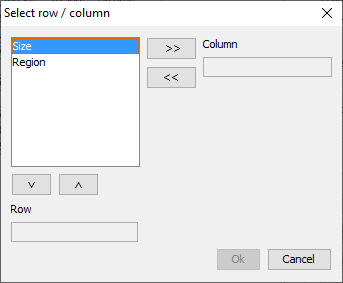 For a 3 dimensional table, this window is as follows:
 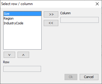 Table summary Pressing 'table summary' provides a table summary giving an overviewof the number of cells according to their status. The example shownhere refers to the case after secondary suppression has beenperformed.
 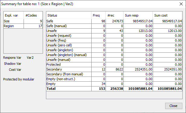 The headings in the summary window are as follows: Freq: The number of cells in each category # rec: The number of observations in each category Sum resp: Total cell value in each category Sum cost: The sum of the cost variable. Hor. Levels and Vert. levels A large (hierarchical) table can never be showncompletely on the screen. Therefor \(\tau\)-Argus will start by showing onlythe top-2 levels of the hierarchy. With these options you can specifythat more levels of the table must be shown. Alternatively you can click on the + and – symbols ofthe hierarchical codes in the table to fold and unfold parts of thetable. ****3 dig separator**** This removes or inserts the character separating the thousands for thevalues in the table. Output View This option allows the table to be shown as it will be output, withsuppressed cells (primary and secondary) replaced by a X.

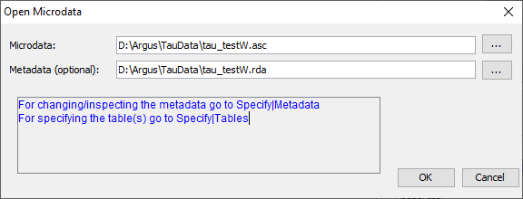 In this dialog box the user can select the microdata-file or the SPSSsystem file and optionally the corresponding metadata file By default the microdata-file has extension .asc and the metafile.rda. .(Note, the user may use any file extension, but is advised touse default names).
  When the user clicks on he will get the traditionalopen file dialog box.
 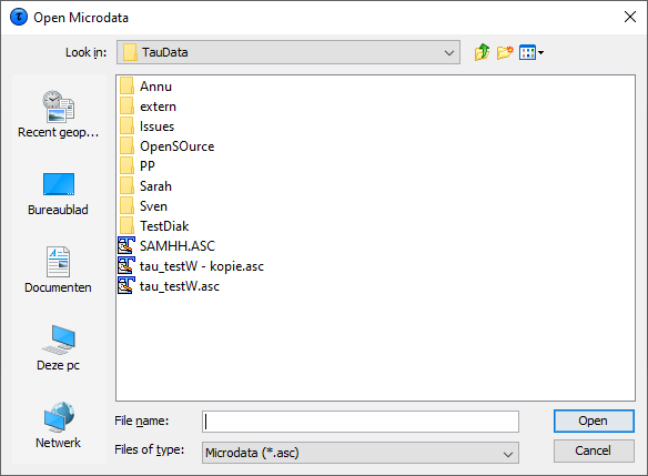 This box enables searching for the required files. Otherfile-extensions can be chosen when clicking on the files of typelistbox. When the user has selected the microdata file a suggestionfor the metafile (with the same name but with the extension .rda) isgiven but only when this file exists. Note, both files do notnecessarily have to have the same name. If a user selects a data file with another extension,
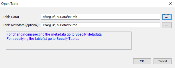 The name of the file containing the table to be opened (in the formatgiven below) needs to be specified in the first line. Optionally thename of the file containing the metadata is entered in the secondline. Later on you will be offered the option of adapting the metadataor even enter the metadata from scratch. There is a great flexibility with this option. The structure of the file is that each line/record describes one cellin free format. The separator is to be specified in the metadata. Themore detail is given for each cell, the more
 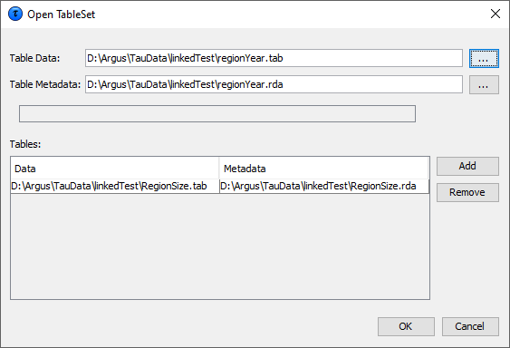 After pressing the OK-button, you will be guided automatically to theSpecify Tables window. This is described in section[4.4.5]. In the linked tables approach it is no longer possible to modify themetadata. As the same rules will be applied to each individual table, you willbe guided to the Specify Tables window only once. The choices will beapplied to each table. This implies that all tables in a linked set should have the sameadditional variables, as described in the previous section[4.3.2]. Please note that it is advisable to read each table individually inτ‑argus before. This to be sure that the specification of the tablesand the metadata is correct, before starting the linked tablesprocedure.
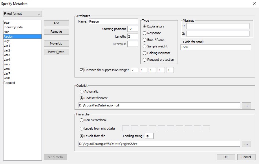 If under File|Open Microdata an rda-file has been specified, thisdialog box shows the contents of this file. If no .rda-file has beenspecified the information can be specified in this dialog box afterpushing the New button. As default "New" is substituted as thevariable name, but the user is expected to fill in a correct name.Apart from defining a new variable, an existing one can be modified ordeleted. In the left top field the file type (fixed, free format or SPSS) canbe specified. The following attributes for each variable can be specified or edited:
 If the RDA-file has been specified too this step is not needed. Extending the metadata Secondly the meta data has to be filled in that could not beautomatically retrieved from the system file. SPSS gives only thebasic information like variable names, field length. But northingabout SDC-specific information The working of
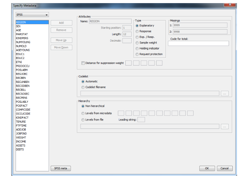
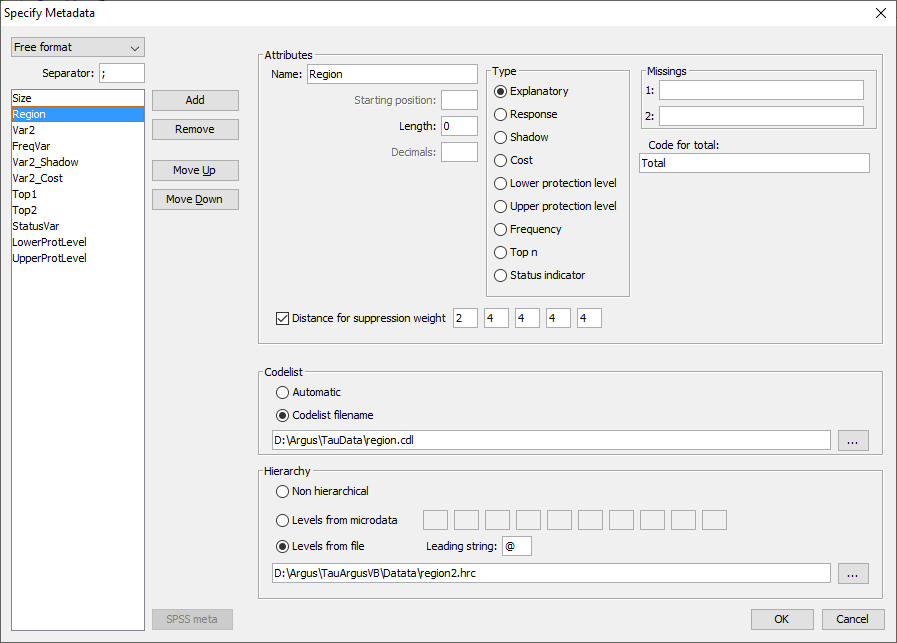 The codelist and the hierarchy are the same as for microdata, so werefer to section [4.4.1]. For explanatory variables the code for the total has to be specified.We strongly recommend strongly that the user also provides the valuesfor the totals himself, but if needed he can ask
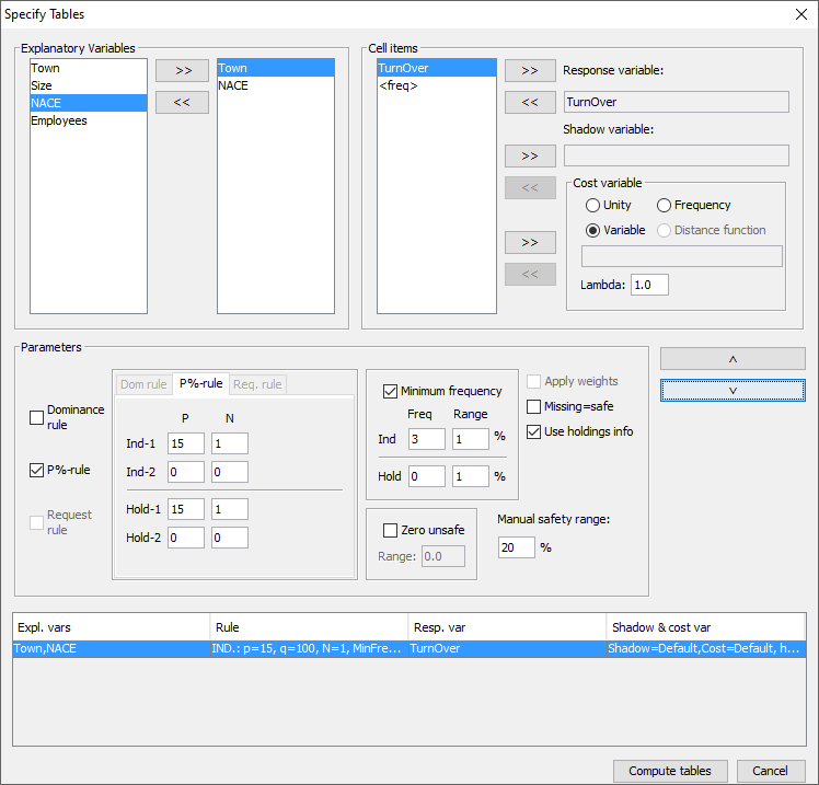
 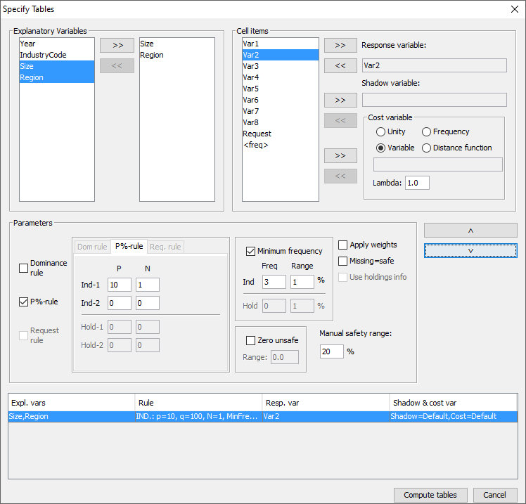 In section [4.4] details of variable definitions in themetafile were explained. Now consider how the variables defined in themetafile are used to create a table along with an associated safetyrule. The explanatory (or spanning) variables On the left is the listbox with the explanatory variables. When the user clicks on ‘>’ or ‘<’ the selected variable istransported to the next box. From the left box with explanatoryvariables the user can select the variables that will be used as thespanning variables in the row or the column of the table. Cell items Here, is a list of variables that can be used as response, shadow orcost variables in the disclosure control. By pressing the '>' or'<' they can be transferred to or from the windows on the right. The response variable From the list of cell items the user can select a variable as aresponse variable. This is the variable for which the table to beprotected is calculated. If <freq> is selected a frequency table will be computed. As theneither dominance rule nor the p% rule are meaningful in thissituation, they cannot be used for frequency tables. The shadow variable The shadow variable is the variable that is used to apply the safetyrule. By default this is the response variable, but it is possible toselect another variable. The safety rules are built on the principleof the characteristics of the largest contributors to a cell. If avariable other than the response variable is a better indicator thisvariable can be used here; e.g. the turnover (a proxy for the size ofthe enterprise) can be a suitable variable to apply the safety rule,although the table is constructed using another (response) variable. The cost variable This variable describes the costs of suppressing each individual cell;these costs are used by the internal workings of the secondarysuppression routines. Note that the choice of the cost variable doesnot have any effect when the hypercube method is used for secondarycell suppression. See 2.7.1 for information about how cell costs aredetermined during execution of the hypercube method. With exception ofthe hypercube method, these costs are minimised when the secondarysuppressed cells are determined. By default, this is the responsevariable but two other choices are possible as well as the use of adifferent response variable. Use the frequency of the cells as a cost-function: this will minimisethe number of records contributing to the cells to be suppressed. The number of cells to be suppressed is minimised, irrespective of thesize of their contributions (Unity option). However this might lead tothe suppression of many marginal. A Box-Cox like-transformation can be applied to the individual valuesof the cost variable before minimisation of the cost function. Thesimplified Box Cox function used here is xλ where x is the costvariable and λ is the transformation parameter. For example if λ = 0.5a square root transformation is used and if λ =0 a log transformationwill be applied. Applying this to the unity-choice is rathermeaningless. Weight If the data file has a sample weight, specified in the metadata, thetable can be computed taking these weights into account. If the ‘Apply Weights’ box is ticked, the weights are applied to thecell entries as for the simple application of normal sampling weightsin a survey. In addition these weights are used in applying the safetyrules. When we have a sample the normal idea behind the sensitivityrules that the largest contributions can make a good estimate of eachother is no longer valid. The solution is that we artificially createa complete cell by assuming that each contribution is in fact as manycontributions as its sample weight. And we apply the sensitivity ruleson this cell. An example might help here. For example if there is a cell with two contributions: 100, weight 4 10, weight 7 The cell value = (4 x 100) + (7 x 10) = 470. Without considering theweights there are only two contributors to the cell 100 and 10.However by taking account of the sampling weights the cell values areapproximately 100, 100, 100, 100, 10, 10, 10, 10, 10, 10 and 10. Thelargest two contributors are now 100 and 100. These are regarded asthe largest two values for application of the safety rules. If theweights are not integers, a simple extension is applied. The safety rule The concept of safety rules is explained in section [2.2]On the left side of the window the type of rule that can be selectedalong with the value of the parameters is shown. The possible rulesare:
 Consider the following dataset
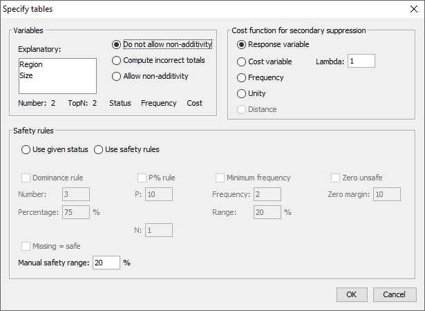
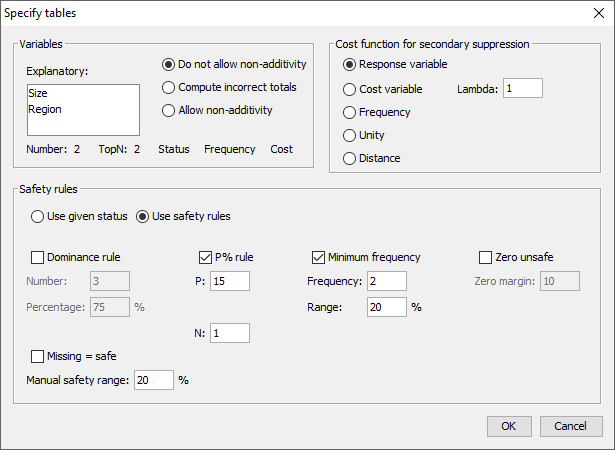 In the safety rule frame, the type of rule can be selected along withthe value of the parameters. These are the dominance rule and P% rule.Additionally, the minimum number of contributors can be chosen(threshold rule), via ticking and filling-in the minimum frequencybox. If both the status and some information to apply the sensitivityrules have been supplied, both options ‘use given status’ and ‘usesafety rules’ are enabled and the user can chose which one to use. Depending one the amount of detail in the table file some options willbe disabled. If no top1 and top2 information is provided, the p%-rulecannot be used. There is an option to calculate the possibly missing marginals andtotals. This option should be used only as an emergency. It is alwaysbetter to provide τ‑argus with a full, complete table. When
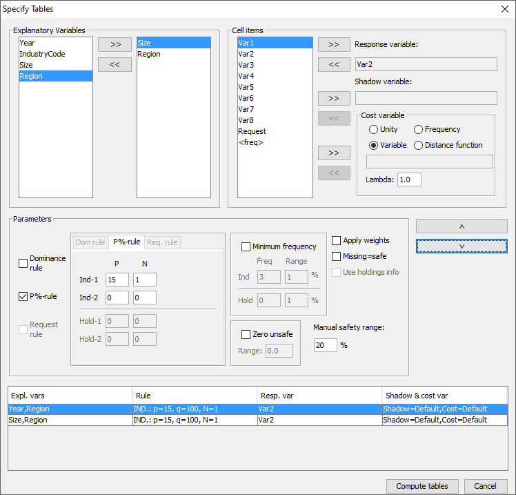 When the tables are supplied to τ‑argus as tabular input see section[4.3.3] (Open Table set). When supplying a set of readymade tables it should be clear to τ‑argus which explanatory variablesare in fact the same dimension. They should have the same name, evenif the level of detail is different. The next step is to further define the tables. This is similar to theprocedure in Specify Tables (see section [4.4.5]). Thesame choices for the parameters etc. are applied to each table. Itwill be clear that all tables should have the same amount of detail.Otherwise the choices cannot be applied to all tables. So it is notpossible that one table just has a Status indicator and another tablehas the top-2 allowing for applying the p%-rule.
  E.g. if a regional variable is an explanatory variable in two tables,but in one table it is at the level of province and in the other atthe level of municipality, they should nevertheless have the samename. If not τ‑argus will not recognise them as a link. The set of linked tables can be protected using the hypercube (seesection [2.8]) and the extended modular approach(see section [2.11]). When protecting a set of linked tables the restriction is that alltables are a sub-set of a theoretical cover table. The cover table isformed by building a table spanned by all explanatory variable fromthe individual tables and using the longest code list for eachdimension. The dimensions are decided by looking for different namesof explanatory variables. As long as the cover table does not have more than 10 dimensions andall the individual tables have not more that 4 dimensions, the linkedtables approach is possible. In the current implementation there is one restriction. For each ofthe spanning variables in the cover table the codelist and thehierarchy should be present in one of the linked tables. For all othertables the codelists and the hierarchy should be a subset of thiscover hierarchy. And of course the set of linked tables should beconsistent. The cells that are logical the same should have exactlythe same value and status. If not the protection of the cover tablewill fail. When tabular data is the starting point, it is the responsibility ofthe user that the tables are consistent. This means that the cellvalues of corresponding cells** **are the same and also the status. Ifnot this is an inconsistent situation. The modular approach is verystrict on complete additivity, as the optimisation routines behindmodular require this. The hypercube is a bit more relaxed.
 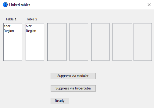 The set of linked tables can now be protected by pressing ‘Suppressvia modular’ or ‘suppress via hypercube’.
  When making the cover table
 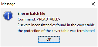 In the example the value of cell “Total,Nr”(4373664.0) and “12,Total” (1441228.0) are not correct. In twodifferent input files the status is not equal.
 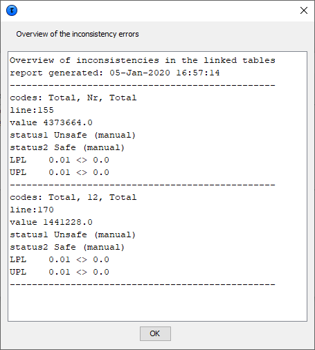 When the hypercube is selected, all the input files for the hypercubewill be prepared and the linked table procedure of the hypercube willbe started to protect the set of tables. Also the hypercube does notlike inconsistencies in e.g. the status. These will be reported in thefile PROTO002 in the temp-directory.
  If successful the following information will be shown:
 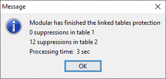 When the protection has been completed, the linked tables procedurecan be closed and the individual protected subtables can be inspectedand stored as normal tables.
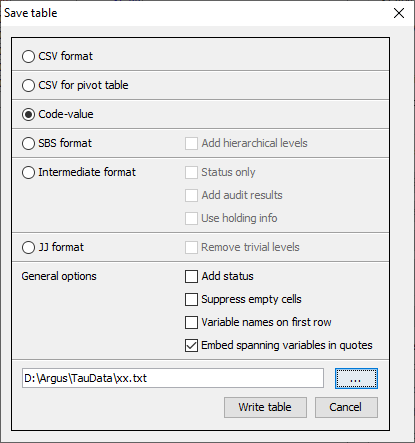 As a CSV file. This Comma Separated file can easily be read intoExcel. Please note the Excel should interpret the comma as aseparator. If your local settings are different you could use theExcel option ‘Data|Text to Columns’, This a typical tabular outputmaintaining the appearance of the table in
 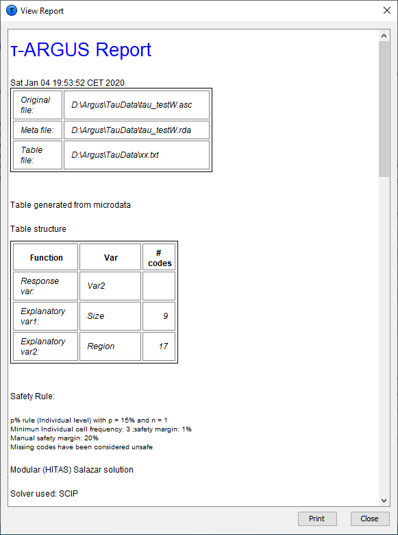 A nicer view of the report will be obtained if you open the report ina web-browser: